When Normal Science fails: a clinical anomaly that opens the problem

File:Bars-icon.svg

Home

Scientific community

Book index

Our network

Frisardi Masticationpedia Network

Fontana Masticationpedia Network

Donate

Contact

Change language

German

Spanish

French

Italian

English

When Normal Science fails: a clinical anomaly that opens the problem

Abstract: This chapter closes the Normal Science phase by examining a central diagnostic vulnerability in Orofacial Pain (OP) and Temporomandibular Disorders (TMD): the risk of mistaking a “TMD-like” clinical presentation for systemic or neurological conditions capable of mimicking it, especially in early stages. Starting from a 5-year prospective clinical follow-up, we introduce the conceptual foundation of the Ψ Index as a diagnostic paradigm oriented toward managing uncertainty, in which the outcome depends not only on “which test” is performed, but also on when and in what order information is acquired.

In a first phase, Bayesian updating is applied to a diagnostic pathway based on RDC/TMD, yielding a high conditional probability of TMD when the RDC output is positive within the symptomatic cohort. However, long-term follow-up reveals that many symptomatic patients initially classified as TMD were in fact carriers of severe non-TMD conditions. This produces an “interference-like” distortion of diagnostic certainty: a quantitative drop from 81% to 9.56% in a contextual model, used here to formalize the epistemological transition from deterministic commutativity to clinical non-commutativity (order effects).

The chapter concludes by arguing that deterministic diagnostic formalism is insufficient in multifactorial conditions, and that future clinical research should explore contextual and quantum-like probabilistic frameworks as tools to model order effects, diagnostic interference, and clinically high-impact uncertainty.

Introduction

We reach the end of the Normal Science section (in Kuhnian terms: a mature phase of “puzzle-solving” under a dominant paradigm), in which the current status quo in OP and TMDs has been presented together with a set of unresolved diagnostic vulnerabilities. These vulnerabilities are not yet “anomalies” in the strict Kuhnian sense, but they are critical points that systematically threaten diagnostic safety and timeliness.

Chronic OP conditions are difficult to diagnose and treat because the mechanisms of etiology and pathogenesis remain only partially understood. A frequent feature of OP is its multifactorial nature: pain related to TMDs often overlaps with symptoms and signs that may also be early manifestations of neurological or systemic diseases, making differential diagnosis complex.

In patients with functional disorders of the stomatognathic system, peripheral risk factors (including occlusal variables) have been reported, as well as central biopsychosocial risk factors involving CNS dysfunction. However, these frameworks have neither resolved causal mechanisms nor generated a decisive improvement in clinical management; consequently, a wide range of predominantly conservative treatments persists.

A relevant obstacle in OP/TMD differential diagnosis remains the instability of standardized criteria to define TMD subtypes, historically addressed through the development of the Research Diagnostic Criteria (RDC). For an overview of RDC, see the dedicated chapter.

The prospective study presented here constitutes the bridge toward the Ψ Index paradigm. The cohort was evaluated longitudinally in three clinically distinct phases:

• $t_0$ — preliminary diagnostic phase
• $t_n$ — advanced diagnostic phase (after follow-up and expert re-evaluation)
• $t_{n+1}$ — definitive diagnostic closure (protocol modeling: Index $|\mathrm{\Psi }⟩$, read “ket Psi Index”)

Since the first step is anchored to Bayesian updating, we recall the minimal formalism.

Bayes' Theorem (minimal recall)

Bayes' theorem updates the probability of a hypothesis in light of evidence:

$P(A|B)=\frac{P(B|A)P(A)}{P(B)}$

where:

• $A$ — hypothesis (e.g., “TMD present”)
• $B$ — evidence (e.g., “RDC output positive”)

and:

$P(B)=P(B|A)P(A)+P(B|\mathrm{\neg }A)(1-P(A))$

Important clinical note: in diagnostic practice, probabilities are often computed on a selected cohort (e.g., symptomatic patients entering a pathway), not on the general population. For this reason, the prevalence $P(A)$ must be defined with respect to the cohort under analysis.

Ψ Index at time $t_0$ (Bayesian certainty in the symptomatic cohort)

At time $t_0$, the RDC model is applied to a sample of 40 subjects (30 asymptomatic, 10 symptomatic). Within the symptomatic cohort, 9 subjects are classified as TMD-positive according to RDC, whereas 1 symptomatic subject is classified as non-TMD according to RDC (Table 1).

To avoid a misleading “population prevalence”, we state explicitly:

• Cohort = symptomatic patients entering the diagnostic pathway (n=10)
• $A$ = “TMD (as classified by the RDC model at time $t_0$)”
• $B$ = “positive RDC test output”

From the cohort:

• $P(A)=\frac{9}{10}=0.9$
• Sensitivity (observational/assumed for the RDC pathway in this cohort): $P(B|A)=0.9$
• Specificity (observed/assumed in this dataset): $P(\mathrm{\neg }B|\mathrm{\neg }A)=1$, hence $P(B|\mathrm{\neg }A)=0$

Then: $P(B)=0.9\cdot 0.9+0\cdot (1-0.9)=0.81$

and: $P(A|B)=\frac{0.9\cdot 0.9}{0.81}=1$

Therefore, in the symptomatic cohort and under these conditions, a positive RDC output produces an apparently “certain” TMD classification.

This is where the epistemological risk emerges: a probabilistic certainty can be produced within a model even when the clinical ground truth (etiology and systemic risk) is not aligned with the model’s hypothetical space.

For example, clinically complex scenarios may mimic OP/TMD patterns and confound classification.

For this reason, symptomatic subjects were re-evaluated by a multidisciplinary team and followed longitudinally. The advanced phase at time $t_n$ changes the diagnostic landscape.

Ψ Index at time $t_n$ (order effects and diagnostic non-commutativity)

Follow-up and expert re-evaluation reveal that many symptomatic subjects were carriers of severe non-TMD pathologies (e.g., meningiomas, pineal cavernomas, scleroderma, hemimasticatory spasm). These conditions were already discussed in the Normal Science chapters, but their occurrence within an “RDC-TMD positive” cohort constitutes genuine epistemological pressure on the paradigm.

Classical diagnostic thinking often assumes commutativity: variables and tests can be permuted without changing meaning. Clinically, however, time creates an order: lesion evolution, symptom emergence, and test sensitivity are time-dependent. Consequently, the order in which information is acquired can modify the diagnostic outcome.

Table 1: RDC output at time $t_0$ on 40 subjects (30 asymptomatic, 10 symptomatic).

Table 2: change in accuracy after follow-up and expert re-evaluation.

Paradigmatic example (prudent): temporal and sequential dependence

A minimal clinical example makes the point intuitive without forcing conclusions: given the same reported symptomatology (bruxism/orofacial pain), the clinical reading can change substantially when time and the order of acquisition of informational blocks change.

• In 2000: a standard dental pathway (RDC-type criteria and tests oriented to the TMD context) produces a locally coherent classification: “TMD/bruxism”.
• In 2014: a neurophysiological work-up, performed at a more advanced phase and with greater discriminative power for some trigeminal conditions, produces data compatible with a different etiological scenario and forces a differential re-evaluation.

Here, the example is not used to claim that a single test “diagnoses” a specific pathology, but to introduce a clinically crucial fact: the diagnostic outcome may depend not only on which information is available, but also on when and in which sequence it is acquired.

Operationally, we can describe the pathway as a sequential application of two blocks:

• $A$ = standard dental block (local TMD/RDC reading)
• $B$ = neurophysiological/systemic block (higher-level, differential reading)

and explicitly admit that between $A$ and $B$ there is a time $T$:

$A\stackrel{T}{\mid }B$

When the system is complex and has overlapping phases, it is not guaranteed at all that inverting the order is neutral:

$D\left(A\stackrel{T}{\mid }B\right)\ne D\left(B\stackrel{T}{\mid }A\right)$

The full formalization of this point (diagnostic non-commutativity as outcome dependence on order and time) is developed in the dedicated chapter: Non-commutative variables in clinical practice.

Why an index of state is needed

The results presented indicate that the diagnostic outcome cannot be adequately represented as a single scalar numerical value. What matters, in complex clinical systems, is not only the intensity of an index, but the overall configuration of the system’s state: modulus, phase, informational orientation, and dependence on the observational path.

A purely scalar model allows data to be ordered along a single dimension (for example “more” or “less” pathological), but it cannot distinguish clinically different states that share the same numerical value. In such cases, equality of value does not imply equivalence of state.

It is in this context that the need emerges for a mesoscopic state index of a vector nature, capable of representing the clinical system as a configuration rather than as a simple binary classification healthy/sick. Such an index describes not only “how much” a phenomenon is present, but “how” it is organized within the observed clinical system. (Figures 1,2)

• 
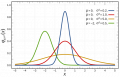  Figure 1: Classical scalar model and probability distribution. In the traditional diagnostic paradigm, clinical information is represented as a numerical value on a one-dimensional line. The bell-shaped distribution does not introduce a new descriptive dimension of the clinical state, but expresses only the frequency of occurrence of a value along the same variable.
• 
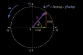  Figure 2: Vector representation of the clinical state (modulus and phase). In the vector model, the state of the clinical system is no longer described by a single scalar value, but by a vector in informational space. The modulus represents the intensity or degree of the observed phenomenon, while the phase encodes the relational configuration and the system’s orientation.

That said, before introducing a vector representation of the clinical state, it is appropriate to examine the operational limits that appear within a classical statistical model consolidated in scientific practice: Bayes' Theorem.

Quantum-like contextual formalization (toy model) — reading guide

Methodological note: the following matrices are a toy model introduced to make the order effect explicit. They are not direct empirical estimates: the coefficients are didactic parameters chosen to make dependence on informational sequence visible.

1) States and state vector

For simplicity we consider two clinical states:

• $S$ = “healthy / absence of evidence of trigeminal hyperexcitability”
• $D$ = “pathological / evidence of trigeminal hyperexcitability”

We represent the patient’s “state” as a vector:

$\psi =\left(\begin{array}{c}p(S)\\ p(D)\end{array}\right)$

where $p(S)$ and $p(D)$ are weights (here treated as probabilities/credence) and satisfy $p(S)+p(D)=1$.

At baseline we assume:

${\psi }_0=\left(\begin{array}{c}1\\ 0\end{array}\right)$ (i.e., initially the system is considered “healthy”).

2) How to read a test-matrix

Each test is represented by a $2\times 2$ matrix that updates the state vector:

${\psi }^{\prime }=\hat{T}\psi$

Reading convention:

• the columns represent the “input” state (before the test),
• the rows represent the “output” state (after the test).

Thus the coefficient $t_{DS}$ indicates how much the test shifts weight from $S$ to $D$.

3) EMG operator $\hat{E}$ (low early discrimination)

We assume an EMG with poor discriminative power in early phases:

$\hat{E}=\left(\begin{array}{cc}0.95& 0.05\\ 0.05& 0.95\end{array}\right)$

Applied to baseline:

$\hat{E}{\psi }_0=\left(\begin{array}{cc}0.95& 0.05\\ 0.05& 0.95\end{array}\right)\left(\begin{array}{c}1\\ 0\end{array}\right)=\left(\begin{array}{c}0.95\\ 0.05\end{array}\right)$

Reading: after EMG the system remains “predominantly healthy” ($p(S)=0.95$), with a small share on $D$ ($p(D)=0.05$).

4) rcIMR operator $\hat{P}$ (high discrimination)

We assume an rcIMR test (recovery cycle of the Masseter Inhibitory Reflex) that is highly discriminative:

$\hat{P}=\left(\begin{array}{cc}0.1& 0.9\\ 0.9& 0.1\end{array}\right)$

Applied to the post-EMG state:

$\hat{P}(\hat{E}{\psi }_0)=\left(\begin{array}{cc}0.1& 0.9\\ 0.9& 0.1\end{array}\right)\left(\begin{array}{c}0.95\\ 0.05\end{array}\right)=\left(\begin{array}{c}0.1\cdot 0.95+0.9\cdot 0.05\\ 0.9\cdot 0.95+0.1\cdot 0.05\end{array}\right)=\left(\begin{array}{c}0.14\\ 0.86\end{array}\right)$

Reading: after rcIMR the weight shifts toward $D$ ($p(D)=0.86$). This makes the order effect visible: the EMG→rcIMR sequence produces a different outcome than the case in which rcIMR is performed as the first test.

5) Scenario 2: rcIMR as the first test

If rcIMR is performed immediately:

$\hat{P}{\psi }_0=\left(\begin{array}{cc}0.1& 0.9\\ 0.9& 0.1\end{array}\right)\left(\begin{array}{c}1\\ 0\end{array}\right)=\left(\begin{array}{c}0.1\\ 0.9\end{array}\right)$

Clinical interpretation: early use of a more discriminative test can make the pathological state emerge sooner, reducing diagnostic delay.

Classical probability vs quantum-like probability (contextual interference)

Classical probability (Kolmogorov, 1933) describes events as sets and assigns to each event a numerical “weight” between 0 and 1.

1) Additivity: what “disjoint events” means

Two events are disjoint when they cannot occur together (they do not overlap). Simple example: in a single draw, “3 occurs” and “5 occurs” are disjoint.

In this case the additive rule holds:

$P(\alpha \cup \beta )=P(\alpha )+P(\beta )$

• $\alpha \cup \beta$ means “$\alpha$ occurs or $\beta$ occurs”.
• Therefore: if $\alpha$ and $\beta$ cannot coexist, the probability of “either one or the other” is the sum of the two.

2) The total probability formula: decomposing a complex problem into simple cases

Often we want to compute the probability of an event $B$ (for example: “test positive”). But $B$ may occur for different reasons: it depends on whether the patient belongs to different classes $A=\alpha$.

The classical total probability formula says:

$P(B=\beta )=\sum _{\alpha }P(A=\alpha )P(B=\beta |A=\alpha )$

Step-by-step reading:

1. $A$ is a variable that separates the possible cases (e.g., clinical classes).
2. $\alpha$ indicates a specific case (a specific class).
3. $P(A=\alpha )$ is how often that case occurs (its frequency/probability).
4. $P(B=\beta |A=\alpha )$ is the probability that we observe $B=\beta$ if we are in the case $A=\alpha$.
5. The sum $\sum _{\alpha }$ means: “I put together all possible cases”.

In other words: → we compute $B$ as a weighted average of the various scenarios $\alpha$.

Classical clinical example: how incidence changes the Bayesian result

Consider a deliberately simple example, drawn from daily clinical practice in TMDs.

Suppose:

• a general population in which the prevalence of TMDs is about 30%

(a figure compatible with many epidemiological estimates).

• a diagnostic test (e.g., RDC-type criteria) with:

* sensitivity $P(B|A)=0.9$

* specificity $P(\mathrm{\neg }B|\mathrm{\neg }A)=0.9$

Where:

• $A$ = “the subject has a TMD”
• $B$ = “the test is positive”

Case 1: general population (prevalence 30%)

Let:

• $P(A)=0.3$
• $P(\mathrm{\neg }A)=0.7$

Compute the probability of a positive test:

$P(B)=P(B|A)P(A)+P(B|\mathrm{\neg }A)P(\mathrm{\neg }A)=0.9\cdot 0.3+0.1\cdot 0.7=0.27+0.07=0.34$

Now the probability that a subject with a positive test truly has a TMD is:

$P(A|B)=\frac{0.9\cdot 0.3}{0.34}\approx 0.79(79\mathrm{\%})$

Case 2: low-prevalence population (prevalence 9%)

Suppose we apply the same test in a population where TMDs are relatively rare (for example, an unselected general population), with prevalence 9%.

Let:

• $P(A)=0.09$
• $P(\mathrm{\neg }A)=0.91$

Compute the probability of a positive test:

$P(B)=P(B|A)P(A)+P(B|\mathrm{\neg }A)P(\mathrm{\neg }A)=0.9\cdot 0.09+0.1\cdot 0.91=0.081+0.091=0.172$

Now compute the probability that a subject with a positive test truly has a TMD:

$P(A|B)=\frac{0.9\cdot 0.09}{0.172}\approx 0.47(47\mathrm{\%})$

Immediate clinical reading

The test is identical to the previous case. Sensitivity and specificity do not change.

Yet:

• with prevalence 30% → $P(A|B)\approx 79\mathrm{\%}$
• with prevalence 9% → $P(A|B)\approx 47\mathrm{\%}$

A “good” test can therefore yield a **clinically weak result** when applied in a low-incidence context.

Simplified clinical reading

The test is **the same**. Sensitivity and specificity do **not** change.

Yet:

• in the general population (example reported in the table on 40 subjects) a positive test means “79% probability of TMD”;
• in the selected population (same example but on 10 symptomatic subjects) it means “93% probability of TMD”.

This shows a key point: diagnostic probability is not a property of the test, but of the **context in which the test is applied**. This means that: for the same test, a positive result does not have an absolute diagnostic meaning, but depends on the population in which the test is applied.

In a low-prevalence TMD population, a positive test provides limited certainty;

in an already selected population, the same result produces much greater certainty.

Already in the classical Bayesian model, therefore, the numerical result depends on the population, selection, and observational history.

Beyond Bayes: when classical probability is not enough

At this point a structural limit of classical Bayesian reasoning emerges, and it is important to make it explicit.

Suppose we are faced with a patient who presents a painful symptomatology fully compatible with a TMD and who, within the standard dental pathway, yields a positive output on the available diagnostic tests. In a classical Bayesian framework, this information tends to progressively increase the posterior probability of the “TMD” hypothesis, especially when the patient belongs to an already selected population.

However, there is a clinically crucial possibility: that the patient does present an odontofacial symptomatology compatible with a TMD, but the true etiology of the pain is different and more severe, for example a neurological pathology such as a pineal cavernoma.

In standard Bayesian formalism, this eventuality can only be handled by expanding the hypothesis space and recomputing probabilities over alternative classes. But in doing so, one implicitly assumes that the different etiological hypotheses contribute independently and additively to the final probability.

The problem is that, in these clinical scenarios, hypotheses are not simply alternatives: they **interact**, compete to explain the same clinical signs, and can produce symptomatic overlaps such that a false sense of diagnostic certainty is generated.

In other words, the presence of a severe non-TMD pathology does not merely add a new hypothesis, but can **reduce** the reliability of the TMD interpretation, even in the presence of positive tests. This effect cannot be represented as a simple subtraction or redistribution of probabilities in the classical model.

This is where the idea of a corrective term is introduced: a contribution that does not sum linearly, but can **attenuate** (or, in other contexts, amplify) the resulting classical probability.

This term, which in the formal language is called “interference”, does not imply any physical transposition of quantum mechanics into medicine. It represents instead a mathematically controlled way to describe the effect of context, etiological competition, and informational order on the diagnostic result.

On these bases it becomes possible to introduce a quantum-like probabilistic formalism, conceived not to replace Bayes, but to extend it in cases where classical probability, even when correctly applied, fails to represent the true instability of the clinical state.

• 
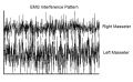  Figure 3: EMG analysis through an interferential pattern model. Only a slight amplitude asymmetry of the motor unit spikes can be noted in the interference trace
• 
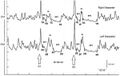  Figure 4: Same patient in whom trigeminal electrophysiological tests were performed, in particular the recovery cycle of the masseter inhibitory reflex
• 
  Figure 5: Definitive diagnosis after 15 years of bruxist symptomatology. Pineal cavernoma

This phenomenon is not a mathematical artifact, but a compact description of a real clinical experience.

3) Why introduce a “quantum-like” term

In complex systems (as in clinical medicine), the outcome may depend on context and on the order in which information is acquired. When this happens, the simple “sum of cases” may not describe well what we observe in practice.

To represent this contextual dependence, a quantum-like formalism introduces a corrective term, called “interference-like”. Attention: here “interference” does not mean there is quantum physics in the patient, but that informational contributions from different cases can combine in a non-purely additive way.

4) The quantum-like formula: same base + a correction

The formula is written as:

$P(B=\beta )=\sum _{\alpha }P(A=\alpha )P(B=\beta |A=\alpha )$

$+$

$+2\sum _{{\alpha }_1<{\alpha }_2}\cos {\theta }_{{\alpha }_1{\alpha }_2}\sqrt{P(A={\alpha }_1)P(B=\beta |A={\alpha }_1)P(A={\alpha }_2)P(B=\beta |A={\alpha }_2)}$

Naive explanation of the additional part

$+2\sum _{{\alpha }_1<{\alpha }_2}\cos {\theta }_{{\alpha }_1{\alpha }_2}\sqrt{P(A={\alpha }_1)P(B=\beta |A={\alpha }_1)P(A={\alpha }_2)P(B=\beta |A={\alpha }_2)}$

• $\sum _{{\alpha }_1<{\alpha }_2}$ means: “I do not sum one case at a time, but I consider pairs of cases”.

(i.e., how two possible classes interact when the context is ambiguous).

• The square root $\sqrt{\cdots }$ is used to build a term that is “symmetric” between the two contributions.

It is a standard way to combine two probabilistic weights without privileging either one.

• $\cos {\theta }_{{\alpha }_1{\alpha }_2}$ is a parameter that modulates the correction:

'if it is positive' the correction increases the final value;

'if it is negative' the correction reduces it;

'if it is zero' the correction vanishes and we return to the classical model.

• The factor $2$ is part of the canonical form of the interferential term: it does not change the conceptual meaning, it only serves to maintain the symmetry of the construction.

In summary:

1. Part 1 is the “standard” total probability. $P(B=\beta )=\sum _{\alpha }P(A=\alpha )P(B=\beta |A=\alpha )$
2. Part 2 adds (or subtracts) a contribution that represents the contextual effect: overlap, ambiguity, informational order, competition between classes. $2\sum _{{\alpha }_1<{\alpha }_2}\cos {\theta }_{{\alpha }_1{\alpha }_2}\sqrt{P(A={\alpha }_1)P(B=\beta |A={\alpha }_1)P(A={\alpha }_2)P(B=\beta |A={\alpha }_2)}$

This is why the model is called “quantum-like”: not because it applies quantum physics to tissues, but because it uses a mathematical structure capable of representing non-additive effects typical of complex systems.

Data from follow-up at time $t_n$ (contextual reinterpretation)

From the follow-up point of view, the symptomatic cohort (n=10) contains:

• subjects initially classified as TMD by RDC at time $t_0$: 9
• subjects subsequently recognized as carriers of severe non-TMD pathologies in the same symptomatic cohort: 7

This indicates that “RDC positive” does not necessarily map onto a “real etiological class” in medically complex OP patients. In other words: the target space of the paradigm is incomplete, and this incompleteness generates a systematic distortion.

We define (for the contextual calculation):

• $P(A={\alpha }_1)=0.9$

probability that a subject in the symptomatic cohort belongs to the “RDC-TMD” class at time $t_0$.

• $P(B=\beta \mid A={\alpha }_1)=0.9$

probability of obtaining a positive RDC output given that the subject belongs to the RDC-TMD class (sensitivity of the RDC pathway in the cohort considered).

• $P(A={\alpha }_2)=0.7$

probability that, following follow-up and expert re-evaluation, a subject in the same symptomatic cohort belongs to a severe non-TMD class (neurological or systemic pathologies with TMD mimicry).

• $\cos \theta =-0.5$

illustrative parameter encoding the diagnostic discrepancy between the two competing etiological readings (${\alpha }_1$ and ${\alpha }_2$).

In this context $\theta$ does not represent a physical angle measured on the patient, but a formal indicator of the degree of conflict between two clinical explanations that produce a similar symptom pattern.

The value $\cos \theta =-0.5$ corresponds to the didactic choice of $\theta =120^{\circ }$, used to represent a “strong but not maximal” negative interference case, in which the presence of a severe non-TMD etiology substantially reduces the diagnostic certainty obtained in the classical model.

True-positive term (classical)

$P_{\text{classical}}=P(A={\alpha }_1)P(B=\beta |A={\alpha }_1)=0.9\cdot 0.9=0.81\to 81\mathrm{\%}$

Corrective “interference-like” term (contextual)

$\mathrm{\Delta }=2\cos \theta \sqrt{0.9\cdot 0.81}\sqrt{0.7}=2(-0.5)\sqrt{0.729}\sqrt{0.7}\approx -0.7144$

Contextual effectiveness

$P_{\text{contextual}}=0.81-0.7144\approx 0.0956\to 9.56\mathrm{\%}$

Interpretation: the RDC pathway can produce a high internal certainty for “TMD classification” while not protecting the patient with respect to severe non-TMD etiologies. The collapse from 81% to 9.56% formalizes the paradigm gap: when the diagnostic space is incomplete, certainty becomes fragile and dependent on the order of information.

A counterintuitive result (but clinically crucial)

The result obtained may appear paradoxical and even unsettling: from an internal Bayesian probability of 81% for TMD classification (within the symptomatic cohort), the contextual model yields an effective probability of about 9.56%.

It is essential to clarify that this “collapse” does not indicate a mathematical error, nor a failure of the RDC test per se. On the contrary, it reveals an epistemological fragility: a high probability can be perfectly coherent **within an incomplete model** and yet be clinically misleading.

In the classical Bayesian model, certainty grows because the “TMD” hypothesis is updated within an etiological space that does not adequately account for alternative pathologies capable of mimicking the symptom profile. The posterior probability correctly answers the question posed by the model, but not necessarily the clinically relevant question.

The introduction of the interference term does not “penalize” TMD: it makes explicit the fact that the same evidence can be shared by competing etiological explanations and that this competition reduces decision safety. In this sense, contextual probability no longer measures the internal coherence of a classification, but its reliability as a clinical guide in the presence of severe alternatives.

The value 9.56% should therefore not be read as a new prevalence estimate, but as an indicator of diagnostic instability: a quantitative signal warning that the decision system is operating in a high-risk overlap region, where numerical certainty does not coincide with clinical safety.

«So, what are we really saying?»

So, what are we really saying?

At this point the reader might legitimately ask: we have shown calculations, probabilities, interferences, matrices, and impressive numerical collapses — but what is the real clinical point of all this?

The point is not to prove that the classical formalism “gets it wrong”, nor to introduce a more sophisticated language for the sake of complexity. The point is simpler and more uncomfortable:

there are clinical contexts in which high numerical certainty does not coincide with a certain diagnosis

The absolute value of an index, even when statistically grounded, is not sufficient to describe the system’s state. The order in which information is acquired matters; the time separating tests matters; the presence of competing etiologies matters. In these scenarios, diagnosis is not a snapshot, but a path-dependent process.

This raises a set of questions that can no longer be avoided:

• does it make sense to rely on a scalar numerical value when the clinical state evolves and reorganizes over time?
• what does “diagnostic certainty” mean if the outcome depends on the order of tests?
• how can we distinguish a correct but late diagnosis from a truly early diagnosis?
• is it possible to represent the clinical state as something richer than a number: a vector, a phase, a configuration?

The Index $|\mathrm{\Psi }⟩$ arises from these questions, not as a definitive answer, but as an operational attempt to give quantitative form to diagnostic instability. Not to replace existing criteria, but to signal when the clinical system is operating in a dangerous overlap region, where the absolute value ceases to be informative and a concept of state becomes necessary.

If the reader has reached this point with a sense of discomfort — the perception that “something does not add up” despite reassuring numbers — then the problem has been posed correctly. The subsequent sections of the Ψ Index will only explore this discomfort systematically

These chapters are not theoretical ornamentation, but the necessary path to formalize the construction of the Index $|\mathrm{\Psi }⟩$ as a clinical tool: collaborative, dynamic, and deliberately not reducible to a single scalar metric.

Bibliography & references